Take Home_Ex02

1. Background

The country of Oceanus has sought FishEye International’s help in identifying companies possibly engaged in illegal, unreported, and unregulated (IUU) fishing. As part of the collaboration, FishEye’s analysts received import/export data for Oceanus’ marine and fishing industries.

With reference to Mini-Challenge 2 of VAST Challenge 2023 and by using appropriate static and interactive statistical graphics methods, we will be helping FishEye to identify companies that may be engaged in illegal fishing.

2. Data Source

The data is taken from the Mini-Challenge 2 of VAST Challenge 2023. mc2_challenge_graph.json file will be used for the purpose of this exercise.

3. Data Preparation

3.1 Install and launching R packages

The code chunk below uses p_load() of pacman package to check if packages are installed in the computer. If they are, then they will be launched into R. The R packages installed are:

pacman::p_load(jsonlite,tidygraph,ggraph,visNetwork,tidyverse,lubridate,igraph,plotly)

3.2 Loading the Data

fromJSON() of jsonlite package is used to import mc2_challenge_graph.json into R environment.

MC2 <- fromJSON("data/mc2_challenge_graph.json")

3.3 Data Wrangling

3.3.1 Extracting the nodes

The code chunk is used to extract nodes data table from mc2_data list object and save the output in a tibble data frame object called mc2_nodes.

#Extract id, shpcountry and rcvcountry and make it as a tibble database. use select to choose the fields you want and reorganise the fields as you want
MC2_nodes <- as_tibble(MC2$nodes) %>%
  select(id, shpcountry, rcvcountry)
head(MC2_nodes)

# A tibble: 6 × 3
  id                                shpcountry rcvcountry
  <chr>                             <chr>      <chr>     
1 AquaDelight Inc and Son's         Polarinda  Oceanus   
2 BaringoAmerica Marine Ges.m.b.H.  <NA>       <NA>      
3 Yu gan  Sea spray GmbH Industrial Oceanus    Oceanus   
4 FlounderLeska Marine BV           <NA>       <NA>      
5 Olas del Mar Worldwide            Oceanus    Oceanus   
6 French Crab S.p.A. Worldwide      Kondanovia Utoporiana

Things to learn

select() is used not only to select the field needed but also to re-organise the sequence of the fields.

3.3.2 Extracting the edges

The code chunk is used to extract edges data table from mc2_data list object and save the output in a tibble data frame object called mc2_edges.

MC2_edges <- as_tibble(MC2$links) %>%
  select(source, target, arrivaldate, hscode, valueofgoods_omu, valueofgoodsusd, volumeteu, weightkg)

3.3.3 Reviewing the imported data

Next, we will examine the structure of the data frame using glimpse() of dplyr.

glimpse(MC2_nodes)

Rows: 34,576
Columns: 3
$ id         <chr> "AquaDelight Inc and Son's", "BaringoAmerica Marine Ges.m.b…
$ shpcountry <chr> "Polarinda", NA, "Oceanus", NA, "Oceanus", "Kondanovia", NA…
$ rcvcountry <chr> "Oceanus", NA, "Oceanus", NA, "Oceanus", "Utoporiana", NA, …

glimpse(MC2_edges)

Rows: 5,464,378
Columns: 8
$ source           <chr> "AquaDelight Inc and Son's", "AquaDelight Inc and Son…
$ target           <chr> "BaringoAmerica Marine Ges.m.b.H.", "BaringoAmerica M…
$ arrivaldate      <chr> "2034-02-12", "2034-03-13", "2028-02-07", "2028-02-23…
$ hscode           <chr> "630630", "630630", "470710", "470710", "470710", "47…
$ valueofgoods_omu <dbl> 141015, 141015, NA, NA, NA, NA, NA, NA, NA, NA, NA, N…
$ valueofgoodsusd  <dbl> NA, NA, NA, NA, NA, NA, 87110, 188140, NA, 221110, 58…
$ volumeteu        <dbl> 0, 0, 0, 0, 0, 0, 0, 0, 0, 0, 0, 0, 0, 0, 0, 0, 0, 0,…
$ weightkg         <int> 4780, 6125, 10855, 11250, 11165, 11290, 9000, 19490, …

Warning

The output report of MC2_edges above reveals that the arrivaldate is treated as data type instead of date data type. This is an error! Before we continue, it is important for us to change the data type of arrivaldate field to “Date”” data type.

3.3.4 Wrangling Time

MC2_edges <- MC2_edges %>%
  mutate(ArrivalDate = ymd(arrivaldate)) %>%
  mutate(Year = year(ArrivalDate)) %>%
  mutate(Month = month(ArrivalDate)) %>%
  mutate(Monthyear = paste(Year, Month, sep = "-")) %>%
  select(source, target, ArrivalDate, Month, Year, hscode, valueofgoods_omu, volumeteu, weightkg, valueofgoodsusd) %>%
  distinct()
head(MC2_edges)

# A tibble: 6 × 10
  source        target ArrivalDate Month  Year hscode valueofgoods_omu volumeteu
  <chr>         <chr>  <date>      <dbl> <dbl> <chr>             <dbl>     <dbl>
1 AquaDelight … Barin… 2034-02-12      2  2034 630630           141015         0
2 AquaDelight … Barin… 2034-03-13      3  2034 630630           141015         0
3 AquaDelight … -15045 2028-02-07      2  2028 470710               NA         0
4 AquaDelight … -15045 2028-02-23      2  2028 470710               NA         0
5 AquaDelight … -15045 2028-09-11      9  2028 470710               NA         0
6 AquaDelight … -15045 2028-10-09     10  2028 470710               NA         0
# ℹ 2 more variables: weightkg <int>, valueofgoodsusd <dbl>

Things to learn

• mutate() is used 4 times to create 4 derive fields.

  • ymd() of lubridate package is used to covert arrivaldate field from character data type into date data type.

  • year() of lubridate package is used to convert the values in ArrivalDate field into year values.

  • month() of lubridate package is used to convert the values in ArrivalDate field into month values.

• select() is used not only to select the field needed but also to re-organise the sequent of the fields.

3.3.5 Checking if there is any missing values in the edge data table

The below chunck is used to calculate the percentage of NAs and 0s in the each column in the edge data table to see if we should use it for our analysis.

# Select specific columns in your dataset
selected_columns <- c("valueofgoods_omu", "volumeteu", "weightkg", "valueofgoodsusd")

## Calculate the percentage of NA values and zeros for the selected columns
total_rows <- nrow(MC2_edges)
na_percentage <- colSums(is.na(MC2_edges[, selected_columns])) / total_rows * 100
zero_percentage <- colSums(MC2_edges[, selected_columns] == 0, na.rm = TRUE) / total_rows * 100

# Combine the results into a data frame
result <- data.frame(NA_Percentage = na_percentage, Zero_Percentage = zero_percentage)

# Display the result
result

                 NA_Percentage Zero_Percentage
valueofgoods_omu      99.99471      0.00000000
volumeteu              9.38167     75.91084870
weightkg               0.00000      0.90128491
valueofgoodsusd       54.36443      0.08169013

Warning

There is a high percentage of NA value in valueofgoods_omu and valueofgoodusd and a high percentage of zero in volumeteu, thus we will leave them out in our analysis, since we are unable to derive any useful insights.

3.3.6 Preparing the edges data table

Harmonized System (HS) codes are the identification codes given to goods for use in international trade. The HS codes are administered by the World Customs Organization (WCO) and are internationally accepted for use by customs authorities and companies to identify goods.

Since we are doing an analysis on the fishing industry, we have to first filter those hscodes that are fishing industry related products.

mc2_edges_aggregated <- MC2_edges %>%
  filter(grepl("^30[1-8]|^2301|^160[4-5]|^1212|^1302|^1504|^151610|^151790", hscode)) %>% # filter out only those hscode that are fishing industry related products 
  group_by(source, target, hscode, Year) %>%
    summarise(weights = n(), median_weight = median(weightkg)) %>%
  filter(source!=target) %>%
  filter(weights>10) %>%
  ungroup()
mc2_edges_aggregated

# A tibble: 12,408 × 6
   source                              target hscode  Year weights median_weight
   <chr>                               <chr>  <chr>  <dbl>   <int>         <dbl>
 1 " Direct Herring Company Transit"   Estre… 306170  2031      12        21078.
 2 "1 Limited Liability Company"       Olas … 303630  2034      28        19830 
 3 "1 Limited Liability Company Trans… Selou… 160414  2030      12         9985 
 4 "1 Limited Liability Company Trans… Selou… 160414  2031      21         8815 
 5 "1 Limited Liability Company Trans… Selou… 160414  2032      16         6908.
 6 "1 Limited Liability Company Trans… Selou… 160414  2033      54         6922.
 7 "1 Limited Liability Company Trans… Selou… 160414  2034      28         6545 
 8 "1 Ltd. Liability Co Cargo"         Himac… 306170  2028      68        10095 
 9 "1 Ltd. Liability Co Cargo"         Himac… 306170  2029      59        19205 
10 "1 Ltd. Liability Co Cargo"         Himac… 306170  2030      26        17708.
# ℹ 12,398 more rows

Next, we take a look at what are the top fishing related products that has most transactions.

top_3_hscode <- mc2_edges_aggregated %>%
  group_by(hscode) %>%
  summarise(total_weights = sum(weights)) %>%
  arrange(desc(total_weights)) %>%
  slice_head(n = 3)

top_3_hscode

# A tibble: 3 × 2
  hscode total_weights
  <chr>          <int>
1 306170        122910
2 304620         81075
3 160414         63745

The top 3 hscodes that has most number of transactions are ‘306170’,‘304620’ and ‘160414’. Thus, we will focus our analysis based on these 3 hscodes.

#Filter the mc2_edges_aggregated based on the top 3 hscode
mc2_edges_aggregated_top <- mc2_edges_aggregated %>%
  filter(hscode == "306170"| hscode == "304620"| hscode == "160414")

#mc2_edges_aggregated_top

Things to learn

• filter() is used to select records whereby hscode that fishing industry related products. The selection of hscode is referenced from the link here

• group_by() is used to aggregate values by source, target, hscode, Year.

• summarise() and n() are used to count the aggregated records.

• filter() is then used to perform the below selection,

  • to select all records whereby source are not equal to target

3.3.7 Preparing the nodes data table

Instead of using the nodes data table extracted from mc2_data, we will prepare a new nodes data table by using the source and target fields of mc2_edges_aggregated data table. This is necessary to ensure that the nodes in nodes data tables include all the source and target values. Then we will reference to the MC2_nodes table to get the corresponding shpcountry and rcvcountry values.

id1_aggregated <- mc2_edges_aggregated_top %>%
  select(source) %>%
  rename(id = source)
id2_aggregated <- mc2_edges_aggregated_top %>%
  select(target) %>%
  rename(id = target)
mc2_nodes_extracted_aggregated <- rbind(id1_aggregated, id2_aggregated) %>%
  distinct()

# Join with MC2_nodes by 'id to get the 'shpcountry', and 'rcvcountry'
mc2_nodes_extracted_aggregated <- mc2_nodes_extracted_aggregated %>%
  left_join(MC2_nodes, by = "id")
head(mc2_nodes_extracted_aggregated)

# A tibble: 6 × 3
  id                                                shpcountry rcvcountry 
  <chr>                                             <chr>      <chr>      
1 " Direct Herring Company Transit"                 Mawazam    Coralmarica
2 "1 Limited Liability Company Transport"           Kondanovia Oceanus    
3 "1 Ltd. Liability Co Cargo"                       Mawandia   <NA>       
4 "6 Ltd. Liability Co Transportation"              Marebak    Oceanus    
5 "8 Aquamarine Limited Liability Company Holdings" Marebak    Oceanus    
6 "9 Marine biology Ltd Family"                     Mawazam    <NA>       

3.3.8 Building the tidygraph model

The code chunk below is then used to build the tidy graph data model.

mc2_graph <- tbl_graph(nodes = mc2_nodes_extracted_aggregated,
                       edges = mc2_edges_aggregated_top,
                       directed = TRUE)
mc2_graph

# A tbl_graph: 930 nodes and 4670 edges
#
# A directed acyclic multigraph with 27 components
#
# A tibble: 930 × 3
  id                                                shpcountry rcvcountry 
  <chr>                                             <chr>      <chr>      
1 " Direct Herring Company Transit"                 Mawazam    Coralmarica
2 "1 Limited Liability Company Transport"           Kondanovia Oceanus    
3 "1 Ltd. Liability Co Cargo"                       Mawandia   <NA>       
4 "6 Ltd. Liability Co Transportation"              Marebak    Oceanus    
5 "8 Aquamarine Limited Liability Company Holdings" Marebak    Oceanus    
6 "9 Marine biology Ltd Family"                     Mawazam    <NA>       
# ℹ 924 more rows
#
# A tibble: 4,670 × 6
   from    to hscode  Year weights median_weight
  <int> <int> <chr>  <dbl>   <int>         <dbl>
1     1   543 306170  2031      12        21078.
2     2   544 160414  2030      12         9985 
3     2   544 160414  2031      21         8815 
# ℹ 4,667 more rows

4. Network Metrics Analysis

4.1 Calculating the in, out and total degree centrality of the nodes

Degree centrality is a measure of immediate connection in a network. It could be interpreted as immediate reach in a social network.Eigenvector centrality is a measure that takes into account both the number of connections that a node or an actor has, and the degree of influence that the node’s immediate connections have in the entire network.

We will calculate the in, out and total degree centrality of the nodes, and use mutate() to create new columns to store these values.

Show the code

#| echo: false
#| fig-width: 3
#| fig-height: 3

# Calulate the in, out and total degree centrality and add 3 new columns via mutate() to store the values 
mc2_graph <- mc2_graph %>%
  activate(nodes) %>%
  mutate(
    in_degree_centrality = centrality_degree(mode = "in"),
    out_degree_centrality = centrality_degree(mode = "out"),
    degree_centrality = centrality_degree(mode = "all"),
    eigen_centrality = centrality_eigen()
  ) %>%
  mutate(combined_centrality = degree_centrality * eigen_centrality) %>%
  arrange(desc(combined_centrality)) 
mc2_graph

# A tbl_graph: 930 nodes and 4670 edges
#
# A directed acyclic multigraph with 27 components
#
# A tibble: 930 × 8
  id            shpcountry rcvcountry in_degree_centrality out_degree_centrality
  <chr>         <chr>      <chr>                     <dbl>                 <dbl>
1 "Mar del Est… Merigrad   Oceanus                     400                     0
2 "Caracola de… Puerto Sol Oceanus                     363                     0
3 "hǎi dǎn Cor… Marebak    Oceanus                     337                     0
4 "Costa de la… Alverossia Oceanus                     181                     0
5 "Blue Horizo… Osterivar… <NA>                          0                   108
6 "Sea Breezes… Isliandor  Coralmari…                    0                   117
# ℹ 924 more rows
# ℹ 3 more variables: degree_centrality <dbl>, eigen_centrality <dbl>,
#   combined_centrality <dbl>
#
# A tibble: 4,670 × 6
   from    to hscode  Year weights median_weight
  <int> <int> <chr>  <dbl>   <int>         <dbl>
1   788   158 306170  2031      12        21078.
2   279     7 160414  2030      12         9985 
3   279     7 160414  2031      21         8815 
# ℹ 4,667 more rows

Below code chunk to find out the top 20 id that has a high combined degree and eigenvector centrality score.

Show the code

#| echo: false
#| fig-width: 3
#| fig-height: 3

#Select the top 20 IDs based on centrality value
top_20_ids <- mc2_graph %>%
  activate(nodes) %>%
  as_tibble() %>%
  pull(id) %>%
  head(20)

top_20_ids

 [1] "Mar del Este CJSC"                   "Caracola del Sol Services"          
 [3] "hǎi dǎn Corporation Wharf"           "Costa de la Felicidad Shipping"     
 [5] "Blue Horizon Family &"               "Sea Breezes S.A. de C.V. Freight "  
 [7] "Selous Game Reserve  S.A. de C.V."   "Playa de Arena OJSC Express"        
 [9] "Pao gan SE Seal"                     "Pao gan LC Freight "                
[11] "AquaDelight N.V. Coral Reef"         "Balkan Cat ОАО Transport"           
[13] "Madagascar Coast  AG Freight "       "Shou gan  Oyj Overseas"             
[15] "Lake Tana  & Son's"                  "Daniel Ferry N.V. Transit"          
[17] "Caracola del Este Ltd. Liability Co" "Viento Azul N.V. Distribution"      
[19] "Tripura  Market S.A. de C.V."        "The Sea Turtle GmbH & Co. KG"       

Bsed on the table above, we can see that the top 20 actors with high combined degree and eigen centrality value, include Mar del Este CJSC, Caracola del Sol Services and hǎi dǎn Corporation Wharf.

Things to learn

activate() is used to make the nodes of mc2_graph active to calculate the degree centrality.

mutate() function from the dplyr package is used to add two new columns, in_degree_centrality and out_degree_centrality, to the nodes of the mc2_graph object

4.2 Determining the type of entity the id belongs to

#Specify what entity the id could be 
mc2_graph <- mc2_graph %>%
  mutate(
    node_type = case_when(
      in_degree_centrality == 0 & out_degree_centrality > 0 ~ "vessels",
      in_degree_centrality > 0 & out_degree_centrality == 0 ~ "transshipment",
      in_degree_centrality > 0 & out_degree_centrality > 0 ~ "vessels/transshipment"
    )
  )

4.2.1 Counting number of entities for each business type

Show the code

#| echo: false
#| fig-width: 3
#| fig-height: 3

#Count the how many id belong to each entity
vessels_count <- mc2_graph %>%
  activate(nodes) %>%
  as_tibble() %>%
  filter(node_type == "vessels") %>%
  nrow()

transhipment_count <- mc2_graph %>%
  activate(nodes) %>%
  as_tibble() %>%
  filter(node_type == "transshipment") %>%
  nrow()

both_count <- mc2_graph %>%
  activate(nodes) %>%
  as_tibble() %>%
  filter(node_type == "vessels/transshipment") %>%
  nrow()

# cat("Number of vessels:", vessels_count, "\n")
# cat("Number of transshipment:", transhipment_count, "\n")
# cat("Number of vessels/transshipment:", both_count, "\n")

After cleaning up the data, we have a total of 529 vessels, 388 transshipment and 13 companies that may be either a vessel or transshipment to work with for our analysis.

Note

• If in_degree_centrality == 0, it means that the company is most likely a pure exporter and highly likely a vessel.

• If out_degree_centrality == 0, it means that the company is most likely a pure importer and highly likely involved in transshipment.

• If in_degree_centrality > 0 & out_degree_centrality > 0, the company is most likely both a vessel or transshipment.

4.3 Visualising the network graph with ggraph

Show the code

#| echo: false
#| fig-width: 3
#| fig-height: 3

ggraph(mc2_graph,
       layout = "fr") +
  geom_edge_link(aes(width=weights), 
                 alpha=0.2) +
  geom_node_point(aes(colour = node_type)) +
  theme_graph() +
  labs(title = "Network graph of global transhipment activities")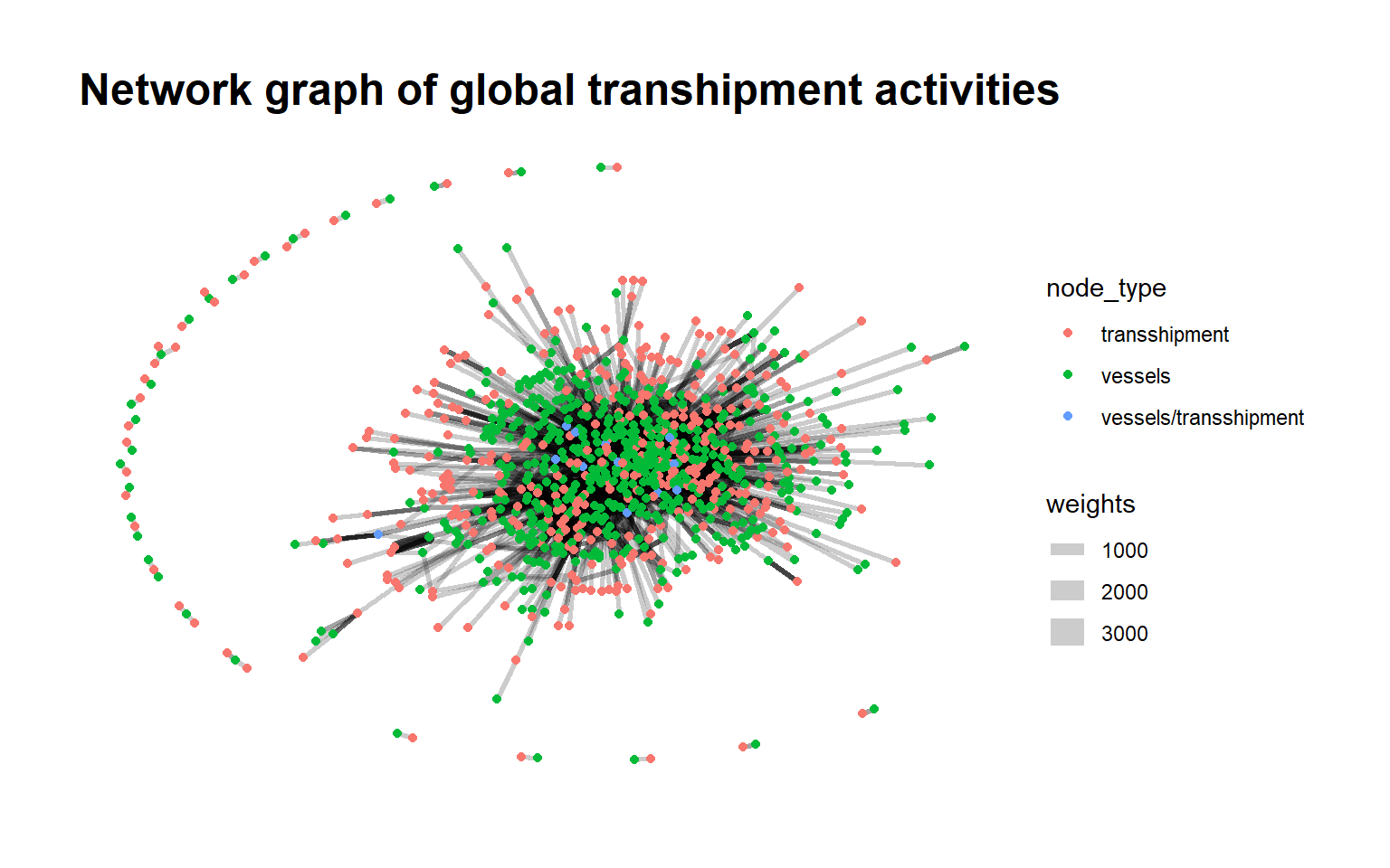

4.4 Flag Based Network

To gain a better understanding of the prevalence of the types of flags in the transshipment events, we can find out which country the vessels tends to be most often associated with when shipping.

And we can see that vessels tend to ship to Merigrad and Marebak.

Show the code

#| echo: false
#| fig-width: 3
#| fig-height: 3

country_id_counts_shp <- mc2_graph %>%
  activate(nodes) %>%
  as_tibble() %>%
  filter(in_degree_centrality == 0) %>% # filter out for the vessels 
  group_by(shpcountry) %>%
  summarise(id_count = n_distinct(id)) %>%
  arrange(desc(id_count))

head(country_id_counts_shp)

# A tibble: 6 × 2
  shpcountry   id_count
  <chr>           <int>
1 Merigrad           97
2 Marebak            78
3 Vesperanda         54
4 Mawazam            52
5 Osterivaria        49
6 Arreciviento       31

Also, we can see that for transshipment, companies are most often associated with Oceanus when receiving their products.

Show the code

#| echo: false
#| fig-width: 3
#| fig-height: 3

country_id_counts_rcv <- mc2_graph %>%
  activate(nodes) %>%
  as_tibble() %>%
  filter(out_degree_centrality == 0) %>% # filter out for the vessels 
  group_by(rcvcountry) %>%
  summarise(id_count = n_distinct(id)) %>%
  arrange(desc(id_count))

head(country_id_counts_rcv)

# A tibble: 6 × 2
  rcvcountry   id_count
  <chr>           <int>
1 Oceanus           362
2 Coralmarica        13
3 Sol y Oceana        5
4 Utoporiana          2
5 Icarnia             1
6 Kethilim            1

4.5 Top 20 transshipment companies trading frequencies

Check out the trading frequencies of the top 20 transshipment companies trading frequencies over the years. These top 20 companies are those who has high in-degree centrality.

We can see that the total transactions fluctuates more for Caracola del Sol Services, Mar del Este CJSC and Pao gan SE Seal.

Show the code

#| echo: false
#| fig-width: 3
#| fig-height: 3

#Select the top 20 IDs based on centrality value
top_20_ids <- mc2_graph %>%
  activate(nodes) %>%
  as_tibble() %>%
  arrange(desc(in_degree_centrality)) %>%
  pull(id) %>%
  head(20)

# Filter the mc2_edges_aggregated_top dataframe
filtered_edges_entities <- mc2_edges_aggregated_top %>%
  filter(target %in% top_20_ids) %>%
  group_by(Year, target) %>%
  summarise(total_weight = sum(weights))

# Plot the aggregated weights
p <- ggplot(filtered_edges_entities, aes(x = Year, y = total_weight, color = target)) +
  geom_line() +
  geom_point() +
  labs(x = "Year", y = "Total transactions", title = "Number of Transactions by Year") +
  scale_color_discrete(name = "Target Entity")

ggplotly(p)

4.6 Community Detection Analysis

Next, we will do a community detection analysis using the group_edge_betweenness function. It works by iteratively removing the edges with the highest betweenness centrality, which is a measure of the number of shortest paths that pass through an edge. By removing these edges, the graph is divided into clusters or communities.

Show the code

#| echo: false
#| fig-width: 3
#| fig-height: 3

set.seed(123)
mc2_graph <- mc2_graph %>%
   mutate(community = as.factor(group_edge_betweenness(weights = weights, directed = TRUE)))

g_mcgraph <- mc2_graph %>%
  activate(nodes) %>%
  group_by(community) %>%
  filter(n() > 2) %>%    #filter the community size > 2
  ungroup() %>%
  ggraph(layout = "fr") + 
  geom_edge_link(aes(width = weights), 
                 alpha = 0.2,
                 arrows = "to") +
  scale_edge_width(range = c(0.1, 5)) +
  geom_node_point(aes(colour = community)) +
  theme_graph()

g_mcgraph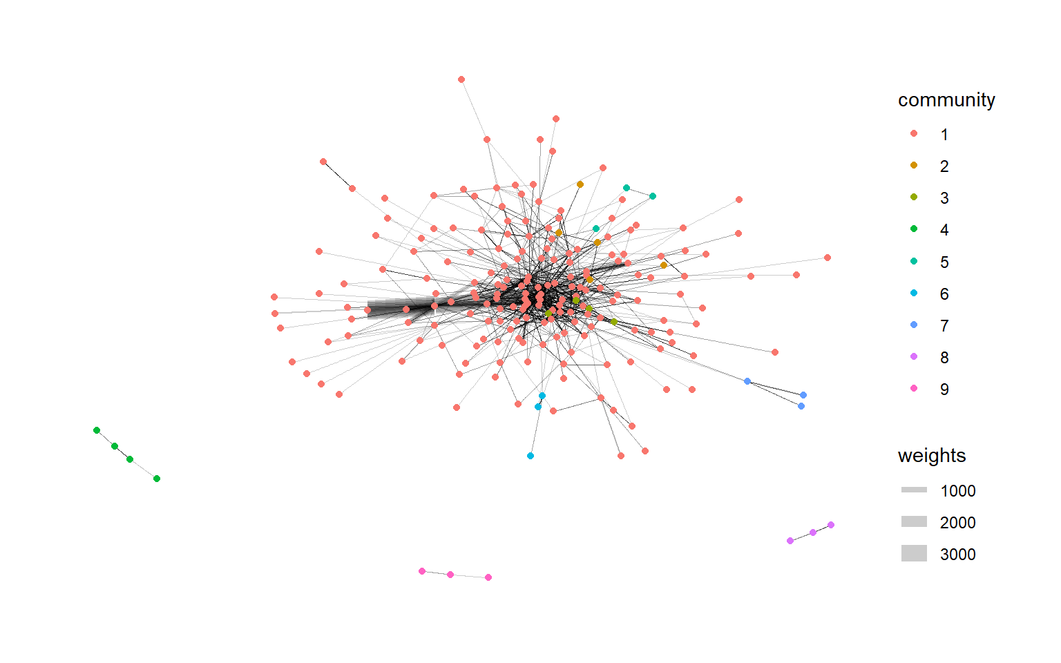

As seen from the community detection graph above, after filtering for community size > 2, there are 9 community shown, and looking at the connectivity and density of the graph, it seems that community 1, seems to be the most densely populated. Thus, for the following analysis, we shall focus on community 1.

The code chunk below can be used to find out which node has the highest in-degree centrality for in community 1. And we can see that within community 1, Mar del Este CJSC has the highest in-degree centrality score.

Show the code

#| echo: false
#| fig-width: 3
#| fig-height: 3

indegree_community <- mc2_graph %>%
  activate(nodes) %>%
  filter(community == 1) %>%
  mutate(in_degree_centrality_community = centrality_degree(mode = "in")) %>%
  arrange(desc(in_degree_centrality_community)) %>%
  as_tibble()

head(indegree_community, 5)

# A tibble: 5 × 11
  id            shpcountry rcvcountry in_degree_centrality out_degree_centrality
  <chr>         <chr>      <chr>                     <dbl>                 <dbl>
1 Mar del Este… Merigrad   Oceanus                     400                     0
2 hǎi dǎn Corp… Marebak    Oceanus                     337                     0
3 Caracola del… Puerto Sol Oceanus                     363                     0
4 Costa de la … Alverossia Oceanus                     181                     0
5 Pao gan SE S… Alverossia Oceanus                     150                     0
# ℹ 6 more variables: degree_centrality <dbl>, eigen_centrality <dbl>,
#   combined_centrality <dbl>, node_type <chr>, community <fct>,
#   in_degree_centrality_community <dbl>

4.7 Plotting the visNetwork graph of transshipment leader

Next, we will further investigate our highest transshipment node, Mar del Este CJSC, by plotting its network graph over the years from 2028-2034 to see if we can find any insights.

2028

Show the code

#| echo: false
#| fig-width: 3
#| fig-height: 3

# Filter the year and id in edges and the corresponding id
filtered_graph_2028 <- mc2_graph %>%
  activate(edges) %>%
  filter(Year == 2028, to == 1)

unique_ids_2028 <- unique(c(filtered_graph_2028 %>%
                         activate(edges) %>%
                         pull(from),
                       filtered_graph_2028 %>%
                         activate(edges) %>%
                         pull(to)))

filtered_graph_2028 <- filtered_graph_2028 %>%
  activate(nodes) %>%
  filter(row_number() %in% unique_ids_2028) %>%
  as_tbl_graph()

edges_df_2028 <- filtered_graph_2028 %>%
  activate(edges) %>%
  as_tibble()

nodes_df_2028 <- filtered_graph_2028 %>%
  activate(nodes) %>%
  as_tibble() %>%
  rename(label = id) %>%
  mutate(id=row_number()) %>%
  select(everything()) %>%
  relocate(id, .before = label)

nodes_df_2028<- nodes_df_2028 %>%
  rename(group = node_type) 

# Plot the network graph with labeled nodes using visNetwork
vis_2028 <- visNetwork(nodes_df_2028, edges_df_2028, submain = list(text = "Network Graph of Mar del Este CJSC in 2028 ",
                          style = "font-family:Comic Sans MS;color:#000000;font-size:15px;text-align:center;")) %>%
  visIgraphLayout(layout = "layout_with_fr") %>%
  visEdges(arrows = "to") %>%
  visOptions(
    highlightNearest = TRUE,
    nodesIdSelection = TRUE,
  ) %>%
  visLegend() %>%
  visInteraction(zoomView = TRUE, dragNodes = TRUE, dragView = TRUE, navigationButtons = TRUE)
vis_2028

2029

Show the code

#| echo: false
#| fig-width: 3
#| fig-height: 3

# Filter the year and id in edges and the corresponding id
filtered_graph_2029 <- mc2_graph %>%
  activate(edges) %>%
  filter(Year == 2029, to == 1)

unique_ids_2029 <- unique(c(filtered_graph_2029 %>%
                         activate(edges) %>%
                         pull(from),
                       filtered_graph_2029 %>%
                         activate(edges) %>%
                         pull(to)))

filtered_graph_2029 <- filtered_graph_2029 %>%
  activate(nodes) %>%
  filter(row_number() %in% unique_ids_2029) %>%
  as_tbl_graph()

edges_df_2029 <- filtered_graph_2029 %>%
  activate(edges) %>%
  as_tibble()

nodes_df_2029 <- filtered_graph_2029 %>%
  activate(nodes) %>%
  as_tibble() %>%
  rename(label = id) %>%
  mutate(id=row_number()) %>%
  select(everything()) %>%
  relocate(id, .before = label)

nodes_df_2029<- nodes_df_2029 %>%
  rename(group = node_type) 

# Plot the network graph with labeled nodes using visNetwork
vis_2029 <- visNetwork(nodes_df_2029, edges_df_2029, submain = list(text = "Network Graph of Mar del Este CJSC in 2029 ",
                          style = "font-family:Comic Sans MS;color:#000000;font-size:15px;text-align:center;")) %>%
  visIgraphLayout(layout = "layout_with_fr") %>%
  visEdges(arrows = "to") %>%
  visOptions(
    highlightNearest = TRUE,
    nodesIdSelection = TRUE,
  ) %>%
  visLegend() %>%
  visInteraction(zoomView = TRUE, dragNodes = TRUE, dragView = TRUE, navigationButtons = TRUE)
vis_2029

2030

Show the code

#| echo: false
#| fig-width: 3
#| fig-height: 3

filtered_graph_2030 <- mc2_graph %>%
  activate(edges) %>%
  filter(Year == 2030, to == 1)

unique_ids_2030 <- unique(c(filtered_graph_2030 %>%
                         activate(edges) %>%
                         pull(from),
                       filtered_graph_2030 %>%
                         activate(edges) %>%
                         pull(to)))

filtered_graph_2030 <- filtered_graph_2030 %>%
  activate(nodes) %>%
  filter(row_number() %in% unique_ids_2030) %>%
  as_tbl_graph()

edges_df_2030 <- filtered_graph_2030 %>%
  activate(edges) %>%
  as_tibble()

nodes_df_2030 <- filtered_graph_2030 %>%
  activate(nodes) %>%
  as_tibble() %>%
  rename(label = id) %>%
  mutate(id=row_number()) %>%
  select(everything()) %>%
  relocate(id, .before = label)

nodes_df_2030<- nodes_df_2030 %>%
  rename(group = node_type) 

# Plot the network graph with labeled nodes using visNetwork
vis_2030 <- visNetwork(nodes_df_2030, edges_df_2030, submain = list(text = "Network Graph ofMar del Este CJSC in 2030 ",
                          style = "font-family:Comic Sans MS;color:#000000;font-size:15px;text-align:center;")) %>%
  visIgraphLayout(layout = "layout_with_fr") %>%
  visEdges(arrows = "to") %>%
  visOptions(
    highlightNearest = TRUE,
    nodesIdSelection = TRUE,
  ) %>%
  visLegend() %>%
  visInteraction(zoomView = TRUE, dragNodes = TRUE, dragView = TRUE, navigationButtons = TRUE) 
vis_2030

2031

Show the code

#| echo: false
#| fig-width: 3
#| fig-height: 3

filtered_graph_2031 <- mc2_graph %>%
  activate(edges) %>%
  filter(Year == 2031, to == 1)

unique_ids_2031 <- unique(c(filtered_graph_2031 %>%
                         activate(edges) %>%
                         pull(from),
                       filtered_graph_2031 %>%
                         activate(edges) %>%
                         pull(to)))

filtered_graph_2031 <- filtered_graph_2031 %>%
  activate(nodes) %>%
  filter(row_number() %in% unique_ids_2031) %>%
  as_tbl_graph()

edges_df_2031 <- filtered_graph_2031 %>%
  activate(edges) %>%
  as_tibble()

nodes_df_2031 <- filtered_graph_2031 %>%
  activate(nodes) %>%
  as_tibble() %>%
  rename(label = id) %>%
  mutate(id=row_number()) %>%
  select(everything()) %>%
  relocate(id, .before = label)

nodes_df_2031<- nodes_df_2031 %>%
  rename(group = node_type) 

# Plot the network graph with labeled nodes using visNetwork
vis_2031 <- visNetwork(nodes_df_2031, edges_df_2031, submain = list(text = "Network Graph ofMar del Este CJSC in 2031 ",
                          style = "font-family:Comic Sans MS;color:#000000;font-size:15px;text-align:center;")) %>%
  visIgraphLayout(layout = "layout_with_fr") %>%
  visEdges(arrows = "to") %>%
  visOptions(
    highlightNearest = TRUE,
    nodesIdSelection = TRUE,
  ) %>%
  visLegend() %>%
  visInteraction(zoomView = TRUE, dragNodes = TRUE, dragView = TRUE, navigationButtons = TRUE) 
vis_2031

2032

Show the code

#| echo: false
#| fig-width: 3
#| fig-height: 3

filtered_graph_2032 <- mc2_graph %>%
  activate(edges) %>%
  filter(Year == 2032, to == 1)

unique_ids_2032 <- unique(c(filtered_graph_2032 %>%
                         activate(edges) %>%
                         pull(from),
                       filtered_graph_2032 %>%
                         activate(edges) %>%
                         pull(to)))

filtered_graph_2032 <- filtered_graph_2032 %>%
  activate(nodes) %>%
  filter(row_number() %in% unique_ids_2032) %>%
  as_tbl_graph()

edges_df_2032 <- filtered_graph_2032 %>%
  activate(edges) %>%
  as_tibble()

nodes_df_2032 <- filtered_graph_2032 %>%
  activate(nodes) %>%
  as_tibble() %>%
  rename(label = id) %>%
  mutate(id=row_number()) %>%
  select(everything()) %>%
  relocate(id, .before = label)

nodes_df_2032<- nodes_df_2032 %>%
  rename(group = node_type) 

# Plot the network graph with labeled nodes using visNetwork
vis_2032 <- visNetwork(nodes_df_2032, edges_df_2032, submain = list(text = "Network Graph ofMar del Este CJSC in 2032 ",
                          style = "font-family:Comic Sans MS;color:#000000;font-size:15px;text-align:center;")) %>%
  visIgraphLayout(layout = "layout_with_fr") %>%
  visEdges(arrows = "to") %>%
  visOptions(
    highlightNearest = TRUE,
    nodesIdSelection = TRUE,
  ) %>%
  visLegend() %>%
  visInteraction(zoomView = TRUE, dragNodes = TRUE, dragView = TRUE, navigationButtons = TRUE) 
vis_2032

#2033

Show the code

#| echo: false
#| fig-width: 3
#| fig-height: 3

filtered_graph_2033 <- mc2_graph %>%
  activate(edges) %>%
  filter(Year == 2033, to == 1)

unique_ids_2033 <- unique(c(filtered_graph_2033 %>%
                         activate(edges) %>%
                         pull(from),
                       filtered_graph_2033 %>%
                         activate(edges) %>%
                         pull(to)))

filtered_graph_2033 <- filtered_graph_2033 %>%
  activate(nodes) %>%
  filter(row_number() %in% unique_ids_2033) %>%
  as_tbl_graph()

edges_df_2033 <- filtered_graph_2033 %>%
  activate(edges) %>%
  as_tibble()

nodes_df_2033 <- filtered_graph_2033 %>%
  activate(nodes) %>%
  as_tibble() %>%
  rename(label = id) %>%
  mutate(id=row_number()) %>%
  select(everything()) %>%
  relocate(id, .before = label)

nodes_df_2033<- nodes_df_2033 %>%
  rename(group = node_type) 

# Plot the network graph with labeled nodes using visNetwork
vis_2033 <- visNetwork(nodes_df_2033, edges_df_2033, submain = list(text = "Network Graph ofMar del Este CJSC in 2033 ",
                          style = "font-family:Comic Sans MS;color:#000000;font-size:15px;text-align:center;")) %>%
  visIgraphLayout(layout = "layout_with_fr") %>%
  visEdges(arrows = "to") %>%
  visOptions(
    highlightNearest = TRUE,
    nodesIdSelection = TRUE,
  ) %>%
  visLegend() %>%
  visInteraction(zoomView = TRUE, dragNodes = TRUE, dragView = TRUE, navigationButtons = TRUE) 
vis_2033

2034

Show the code

#| echo: false
#| fig-width: 3
#| fig-height: 3

filtered_graph_2034 <- mc2_graph %>%
  activate(edges) %>%
  filter(Year == 2034, to == 1)

unique_ids_2034 <- unique(c(filtered_graph_2034 %>%
                         activate(edges) %>%
                         pull(from),
                       filtered_graph_2034 %>%
                         activate(edges) %>%
                         pull(to)))

filtered_graph_2034 <- filtered_graph_2034 %>%
  activate(nodes) %>%
  filter(row_number() %in% unique_ids_2034) %>%
  as_tbl_graph()

edges_df_2034 <- filtered_graph_2034 %>%
  activate(edges) %>%
  as_tibble()

nodes_df_2034 <- filtered_graph_2034 %>%
  activate(nodes) %>%
  as_tibble() %>%
  rename(label = id) %>%
  mutate(id=row_number()) %>%
  select(everything()) %>%
  relocate(id, .before = label)

nodes_df_2034<- nodes_df_2034 %>%
  rename(group = node_type) 

# Plot the network graph with labeled nodes using visNetwork
vis_2034 <- visNetwork(nodes_df_2034, edges_df_2034, submain = list(text = "Network Graph ofMar del Este CJSC in 2034 ",
                          style = "font-family:Comic Sans MS;color:#000000;font-size:15px;text-align:center;")) %>%
  visIgraphLayout(layout = "layout_with_fr") %>%
  visEdges(arrows = "to") %>%
  visOptions(
    highlightNearest = TRUE,
    nodesIdSelection = TRUE,
  ) %>%
  visLegend() %>%
  visInteraction(zoomView = TRUE, dragNodes = TRUE, dragView = TRUE, navigationButtons = TRUE) 
vis_2034

4.7.1 Summary of the changes of transshipment leader over the years

Below is the code chunk to find if there is any missing nodes or addition of new nodes over the different time period:

Show the code

#| echo: false
#| fig-width: 3
#| fig-height: 3

# Diff 2028-2029 

# Check if all nodes in nodes_df_2028 are present in nodes_df_2029
missing_nodes_1 <- setdiff(nodes_df_2028$id, nodes_df_2029$id)

# Get the corresponding names for the missing nodes
missing_node_names_1 <- nodes_df_2028$label[nodes_df_2028$id %in% missing_nodes_1]

# Identify any new nodes in nodes_df_2029
new_nodes_1 <- setdiff(nodes_df_2029$id, nodes_df_2028$id)

# Get the corresponding names for the missing nodes
new_node_names_1 <- nodes_df_2029$label[nodes_df_2029$id %in% new_nodes_1]

# # Print the missing node names with a comma after each label found
# cat("Missing nodes: ", paste(missing_node_names_1, collapse = ", "), "\n")
# # Print the new node names with a comma after each label found
# cat("New nodes: ", paste(new_node_names_1, collapse = ", "), "\n")


#Diff 2029-2030

# Check if all nodes in nodes_df_2020 are present in nodes_df_2030
missing_nodes_2 <- setdiff(nodes_df_2029$id, nodes_df_2030$id)

# Get the corresponding names for the missing nodes
missing_node_names_2 <- nodes_df_2029$label[nodes_df_2029$id %in% missing_nodes_2]

# Identify any new nodes in nodes_df_2030
new_nodes_2 <- setdiff(nodes_df_2030$id, nodes_df_2029$id)

# Get the corresponding names for the missing nodes
new_node_names_2 <- nodes_df_2030$label[nodes_df_2030$id %in% new_nodes_2]

# # Print the missing node names with a comma after each label found
# cat("Missing nodes: ", paste(missing_node_names_2, collapse = ", "), "\n")
# # Print the new node names with a comma after each label found
# cat("New nodes: ", paste(new_node_names_2, collapse = ", "), "\n")


# Diff 2030-2031

# Check if all nodes in nodes_df_2030 are present in nodes_df_2031
missing_nodes_3 <- setdiff(nodes_df_2030$id, nodes_df_2031$id)

# Get the corresponding names for the missing nodes
missing_node_names_3 <- nodes_df_2030$label[nodes_df_2030$id %in% missing_nodes_3]

# Identify any new nodes in nodes_df_2031
new_nodes_3 <- setdiff(nodes_df_2031$id, nodes_df_2030$id)

# Get the corresponding names for the missing nodes
new_node_names_3 <- nodes_df_2031$label[nodes_df_2031$id %in% new_nodes_3]

# # Print the missing node names with a comma after each label found
# cat("Missing nodes: ", paste(missing_node_names_3, collapse = ", "), "\n")
# # Print the new node names with a comma after each label found
# cat("New nodes: ", paste(new_node_names_3, collapse = ", "), "\n")


# Diff 2031-2032

# Check if all nodes in nodes_df_2031 are present in nodes_df_2032
missing_nodes_4 <- setdiff(nodes_df_2031$id, nodes_df_2032$id)

# Get the corresponding names for the missing nodes
missing_node_names_4 <- nodes_df_2031$label[nodes_df_2031$id %in% missing_nodes_4]

# Identify any new nodes in nodes_df_2032
new_nodes_4 <- setdiff(nodes_df_2032$id, nodes_df_2031$id)

# Get the corresponding names for the missing nodes
new_node_names_4 <- nodes_df_2032$label[nodes_df_2032$id %in% new_nodes_4]

# # Print the missing node names with a comma after each label found
# cat("Missing nodes: ", paste(missing_node_names_4, collapse = ", "), "\n")
# # Print the new node names with a comma after each label found
# cat("New nodes: ", paste(new_node_names_4, collapse = ", "), "\n")


# Diff 2033-2034

# Check if all nodes in nodes_df_2033 are present in nodes_df_2034
missing_nodes_5 <- setdiff(nodes_df_2033$id, nodes_df_2034$id)

# Get the corresponding names for the missing nodes
missing_node_names_5 <- nodes_df_2033$label[nodes_df_2033$id %in% missing_nodes_5]

# Identify any new nodes in nodes_df_2034
new_nodes_5 <- setdiff(nodes_df_2034$id, nodes_df_2033$id)

# Get the corresponding names for the missing nodes
new_node_names_5 <- nodes_df_2034$label[nodes_df_2034$id %in% new_nodes_5]

# # Print the missing node names with a comma after each label found
# cat("Missing nodes: ", paste(missing_node_names_5, collapse = ", "), "\n")
# # Print the new node names with a comma after each label found
# cat("New nodes: ", paste(new_node_names_5, collapse = ", "), "\n")

Year	Findings
2028 and 2029	6 Missing nodes: Caracola Marina Lighthouse A/S Forwading Seashell Seekers Ltd Distribution Zanzibar Archipelago Incorporated International Oceanfront Oasis AS Delivery Playa del Sol Incorporated, Kallianassa Fish AG Solutions TunaTime GmbH & Co. KG Export.
2029 - 2030	5 New nodes: Rift Valley fishery OJSC Enterprises Aqua Azul Oyster BV Freight suō yú Incorporated Seagull bái suō wěn lú Ltd. Corporation Freight Norwegian Fjord Plc Transit
2030 - 2031	13 Missing nodes: Barents Sea Shrimp Plc Haryana Sea Marine ecology Gambia River Ges.m.b.H. & Mar y Viento Ltd. Liability Co Captain Gulf of Tadjoura Corp Shipping Barco de Plata SE Dutch Eel LLC Express Icelandic Cod GmbH & Co. KG Express Rift Valley fishery OJSC Enterprises Aqua Azul Oyster BV Freight suō yú Incorporated Seagull bái suō wěn lú Ltd. Corporation Freight Norwegian Fjord Plc Transit
2031 - 2032	20 New nodes: Isla del Tesoro SE Transport Caracola del Este Incorporated Spanish Anchovy OJSC International SaltSea & Inc Carriers Mar de la Aventura Limited Liability Company Mar de Cristalino OJSC jīn qiāng yú Express Mar y Viento Abalone N.V. Marine conservation Playa de Coral Distribution Marine sanctuary xiǎo xiā A/S Holdings Marine Mates Pic Delivery OceanKing s ship Pic Logistics Lake Kariba GmbH & Co. KG Mar y Viento Ltd. Liability Co Captain AquaBite Limited Liability Company Marine SurfSide GmbH & Co. KG Consulting CoralCrest Limited Liability Company Seabass Black Sea Anchovy NV Mar del Oeste LLC Marine Turkish Salmon LC Barracuda
2032 - 2034	10 Missing nodes: Ob River LLC and Son’s Pez Dorado Inc Freight Ola de la Costa Ges.m.b.H. Marine Adventures Ltd Cod Coral Reef Oyj Solutions Estrella de Mar AB Delivery Greek ermen Kga Freight Black Sea Anchovy NV Mar del Oeste LLC Marine Ola del Este Ltd

Also, we can see from the networkgraph that in 2028, Marine Mates NV Worldwide and ReefRider Foods Lte Corporation Family supplies goods to Mar del Este CSJC but disappears in 2029. And in 2032, there are 2 new suppliers, The Salty Dog Limited Liability Company and Turkish Salmon A/S Marine, however, both disappeared in 2034.

5. References

A. Petrossian,G., Barthuly,B.,C. Sosnowski,M.(2022).Identifying Central Carriers and Detecting Key Communities Within the Global Fish Transshipment Networks. Retrieved June 4, 2032, from https://www.frontiersin.org/articles/10.3389/fmars.2022.798893/full

J. Park,A.,Z. Stamato,S.(2020).Social Network Analysis of Global Transshipment: A Framework for Discovering Illegal Fishing.

Datastorm(nd).visNetowork,an R package for an interactive network visualistion. Retrieved June 4, 2032, from https://datastorm-open.github.io/visNetwork/edges.html

https://tidygraph.data-imaginist.com/index.html https://ona-book.org/vertex-importance.html 6 Vertex Importance and Centrality | Handbook of Graphs and Networks in People Analytics (ona-book.org)